Machine Learning with Monster Hunter World Data
Overview
Monster Hunter World (MHW) is a game where players use unique weapons and armor sets to hunt monsters. The monsters range from relatively harmless large insects to extremely powerful elder dragons. Each monster has unique attacks and qualities, and they are grouped within different monster families (e.g., brute wyverns, fanged wyverns, elder dragons, etc.). While these families are a relatively straighforward way of clustering the monsters, I decided in this post to see if the monsters of MHW could be classified into different categories based on their elemental weaknesses. To do this, I've researched and learned about a simple machine learning algorithm known as K-Means clustering.
K-Means clustering is a form of unsupervised machine learning, where the algorithm is not trained on other data, and the algorithm does not seek to predict some outcome measure. Instead, K-Means clustering attempts to calculate how similar/dissimilar a signle data point is from another. The algorithm repeats this process several times until it finds a solution that maximizes within cluster similarity.
Acknowledgements & Disclaimers: Much thanks to Kiranico for posting this data online which can be found here. I make no arguement here that the method I've chosen is the best for identifing clusters in this data set. Furthermore, I am still new to cluster analysis, and have used this data as a way to practice rudimentary methods. If I commit any severe errors, I would be extremely happy for comments, critiques, or suggestions for better methods (grant.pointon@psych.utah.edu).
Data
The data used for this post comes from Kiranaco's database which can be found in the above link. The data includes elemental weakness values for 52 monsters, as well as their assigned monster family. Here is a quick look at the data.
head(MonsterChart)## # A tibble: 6 x 7
## Monster Family Fire Water Thunder Ice Dragon
## <chr> <chr> <dbl> <dbl> <dbl> <dbl> <dbl>
## 1 Anjanath Brute Wyvern 0 21 9 14 4
## 2 Uragaan Brute Wyvern 0 22 3 13 20
## 3 Radobaan Brute Wyvern 9 9 9 11 14
## 4 Barroth Brute Wyvern 12 40 0 14 9
## 5 Deviljho Brute Wyvern 10 10 20 8 20
## 6 Paolumu Flying Wyvern 19 0 13 8 8Machine Learning: K-Means Analysis
First, I explored the data to investigate how many clusters would likely be appropriate for the data. The first plot below represents an elbow curve plot on the total within sums of squares for 1-10 clusters. In elbow plots, the cluster numer that is located at the 'elbow' of the plot is typically regarded as the ideal number of clusters for the data. The second plot shows the average silhouette width for 1-10 clusters. Each plot suggests that 2 clusters would be the most ideal number of clusters to fit the data.
#MODEL COMPARISONS
  # function to compute total within-cluster sum of square (elbow method)
  fviz_nbclust(MonsterChart[,3:7], kmeans, method = "wss")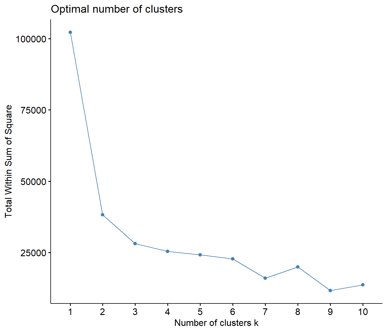
  # silhouette method
  fviz_nbclust(MonsterChart[,3:7], kmeans, method = "silhouette")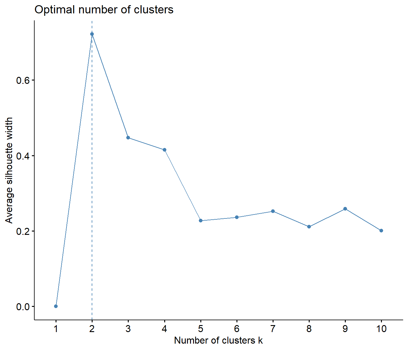
Identifying the ideal number of clusters can also be assessed with the NbClust package, which has a handy function that will run several model fit indices on different cluster solutions. As with the plots above, this handy function also shows that out of 30 model fit indices, 10 suggested that 2 clusters as ideal, 5 suggested 5 clusters as ideal, and 4 suggested 3 clusters as ideal. Therefore, two clusters seems to be the most agreed upon best number of clusters for the data.
  diss_matrix <- dist(MonsterChart[,3:7], method = "euclidean", diag = FALSE)
  NB_clust <- NbClust(MonsterChart[,3:7], diss = diss_matrix, distance = NULL, min.nc = 2,
             max.nc = 10, method = "complete", index = "alllong")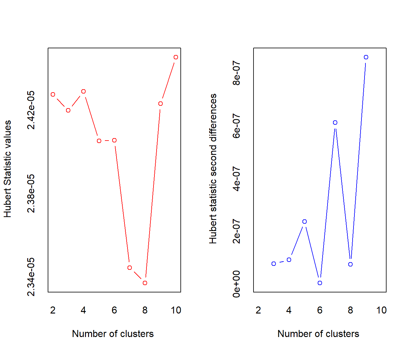
## *** : The Hubert index is a graphical method of determining the number of clusters.
##                 In the plot of Hubert index, we seek a significant knee that corresponds to a
##                 significant increase of the value of the measure i.e the significant peak in Hubert
##                 index second differences plot.
## 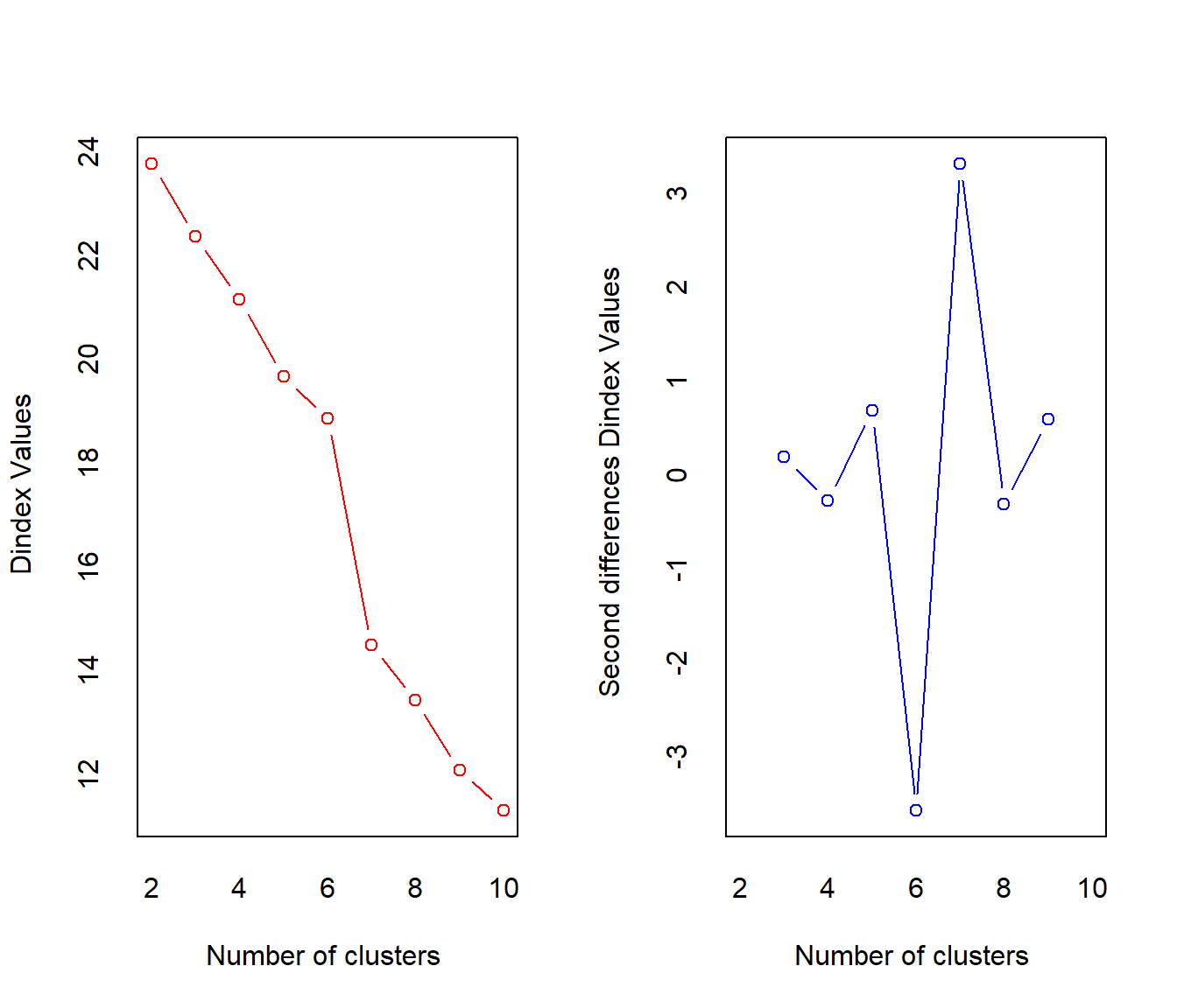
## *** : The D index is a graphical method of determining the number of clusters.
##                 In the plot of D index, we seek a significant knee (the significant peak in Dindex
##                 second differences plot) that corresponds to a significant increase of the value of
##                 the measure.
##
## *******************************************************************
## * Among all indices:
## * 10 proposed 2 as the best number of clusters
## * 4 proposed 3 as the best number of clusters
## * 5 proposed 5 as the best number of clusters
## * 1 proposed 6 as the best number of clusters
## * 4 proposed 7 as the best number of clusters
## * 1 proposed 8 as the best number of clusters
## * 2 proposed 9 as the best number of clusters
## * 1 proposed 10 as the best number of clusters
##
##                    ***** Conclusion *****
##
## * According to the majority rule, the best number of clusters is  2
##
##
## *******************************************************************
Two Cluster Results
Here are the results for the two cluster K-Means analysis. Based off of the best partition using two clusters, it seems that the majority of monsters fall within cluster 1 and only Vespoid, Raphinos, Mosswine, and Kelbi fall into cluster 2.
  #Incorporate cluster partition into data set
  MonsterChart %>%
    mutate(Cluster = NB_clust$Best.partition) %>%
    mutate(Cluster_Name = ifelse(Cluster == 1, "Cluster 1", "Cluster 2")) %>%
    ggplot(aes(x = reorder(Monster, Cluster), y = Cluster_Name)) +
    geom_tile(aes(fill = Cluster_Name), colour = "white") +
    coord_equal(ratio = 0.9) +
    scale_fill_manual(values = c("black", "violet")) +
    theme(axis.text.y = element_blank(),
          axis.text.x = element_text(face = "bold", size = 10, angle = 90, hjust = 1),
            axis.line = element_blank(), axis.title.y = element_blank(), axis.title.x = element_blank(),
            axis.ticks.y = element_blank(), axis.ticks.x = element_blank(),
            axis.ticks.length = unit(0.2, "cm"),
            panel.grid.major = element_blank(), panel.grid.minor = element_blank(),
            panel.border = element_blank(), panel.background = element_blank(),
            legend.title = element_blank(), legend.direction = "horizontal",
            legend.key.size = unit(0.5,"cm"), legend.spacing.x = unit(0.4, "cm"),
            legend.position = c(0.5, 1.5))
Now that we've identified which monsters belong in each of the two clusters, it's time to look more closely and see what sorts of elemental weakness qualities define each of these clusters.
MH_cluster2 <- kmeans(MonsterChart[,3:7],2, nstart = 25)
Cluster2_means <- as.data.frame(MH_cluster2$centers)

Cluster2_means <- Cluster2_means %>%
  mutate(Cluster = c("Cluster 1", "Cluster 2")) %>%
  select(Cluster, Fire, Water, Thunder, Ice, Dragon)

pander(Cluster2_means, style = 'rmarkdown')| Cluster | Fire | Water | Thunder | Ice | Dragon |
|---|---|---|---|---|---|
| Cluster 1 | 12.91 | 14.26 | 15.34 | 15.36 | 11.53 |
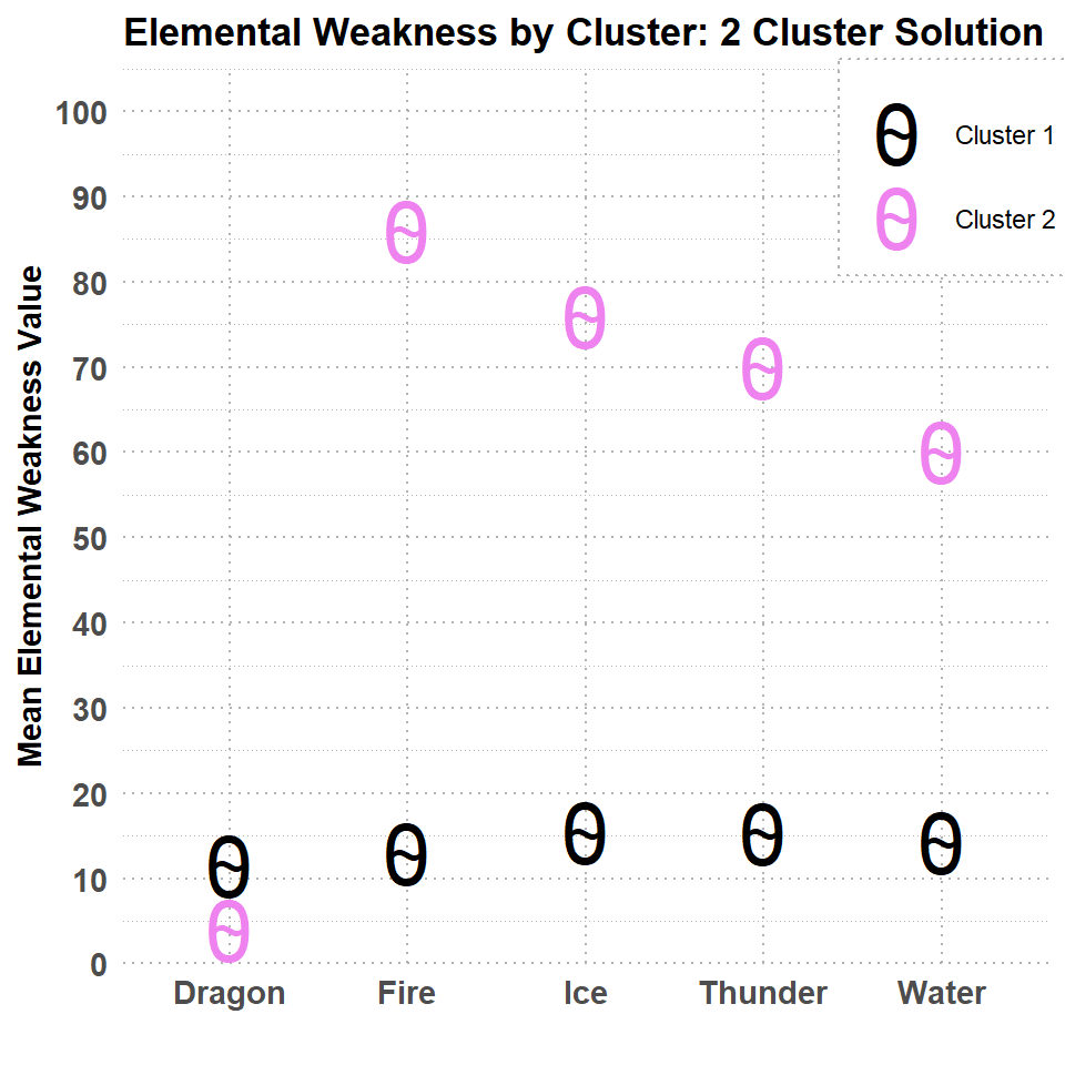
| Cluster 2 | 86 | 60 | 70 | 76 | 4 |
The two clusters seem to reflect a generally low elemental weakness group of monsters and a generally high elemental weakness group of monsters. For an alternative representation, the graph below also shows this pattern of elemental weakness, except with regard to the dragon element.
#Dinasaur egg plot
size1 <- 10
size2 <- size1*0.7
Cluster2_means %>%
  gather(2:6, key = "Element", value = "Cluster Mean") %>%
  ggplot(aes(x = Element, y = `Cluster Mean`, color = Cluster, shape = Cluster)) +
  geom_point(size=size1, shape = 48) +
  geom_point(size=size2, shape = 126) +
  scale_color_manual(values = c("black", "violet")) +
  scale_y_continuous(breaks = seq(0,100,10), limits = c(0,105), expand = c(0,0)) +
  ylab("Mean Elemental Weakness Value") +
  xlab("") +
  ggtitle("Elemental Weakness by Cluster: 2 Cluster Solution") +
  theme_minimal() +
  theme(
    panel.grid = element_line(color = "grey70", linetype = "dotted"),
    legend.position = c(0.9,0.89),
    legend.background = element_rect(fill = "white", color = "grey70", linetype = "dotted"),
   # legend.text = element_text(face = "bold"),
    legend.title = element_blank(),
    axis.text = element_text(face = "bold", size = 11),
      axis.title = element_text(face = "bold"),
   title = element_text(face = "bold")
  )
Two Cluster Conclusion
Based on the results above, it seems like the two cluster solution grouped the monsters into a relatively low elemental weakness group, and a relatively high elemental weakness group. I had originally thought that the cluster analysis would group monsters into about 4-5 clusters because their tends to be groups monsters that share similar primary elemental weaknesses. However, after looking more into the data, there are few monsters who are weak to only one element, and even if they are mostly weak to one element (say fire), their weakness to that element is not of high enough magnitude to really differentiate it from their other elemental weakness values (at least in this data set). Another way to examine this is with a correlation matrix. As can be seen below, the natural elements (fire, water, thunder, ice) are all positively correlated, and quite highly. This further suggests that even if a monster is primarily weak to one natural element, they will likely have increased elemental weaknesses in the other 3 natural elements. There is a possibility, that if the dragon element is excluded from the analysis, that the clustering method would be able to identify more clusters that are specific to each element.
M <- cor(MonsterChart[3:7])
corrplot(M, method = "number")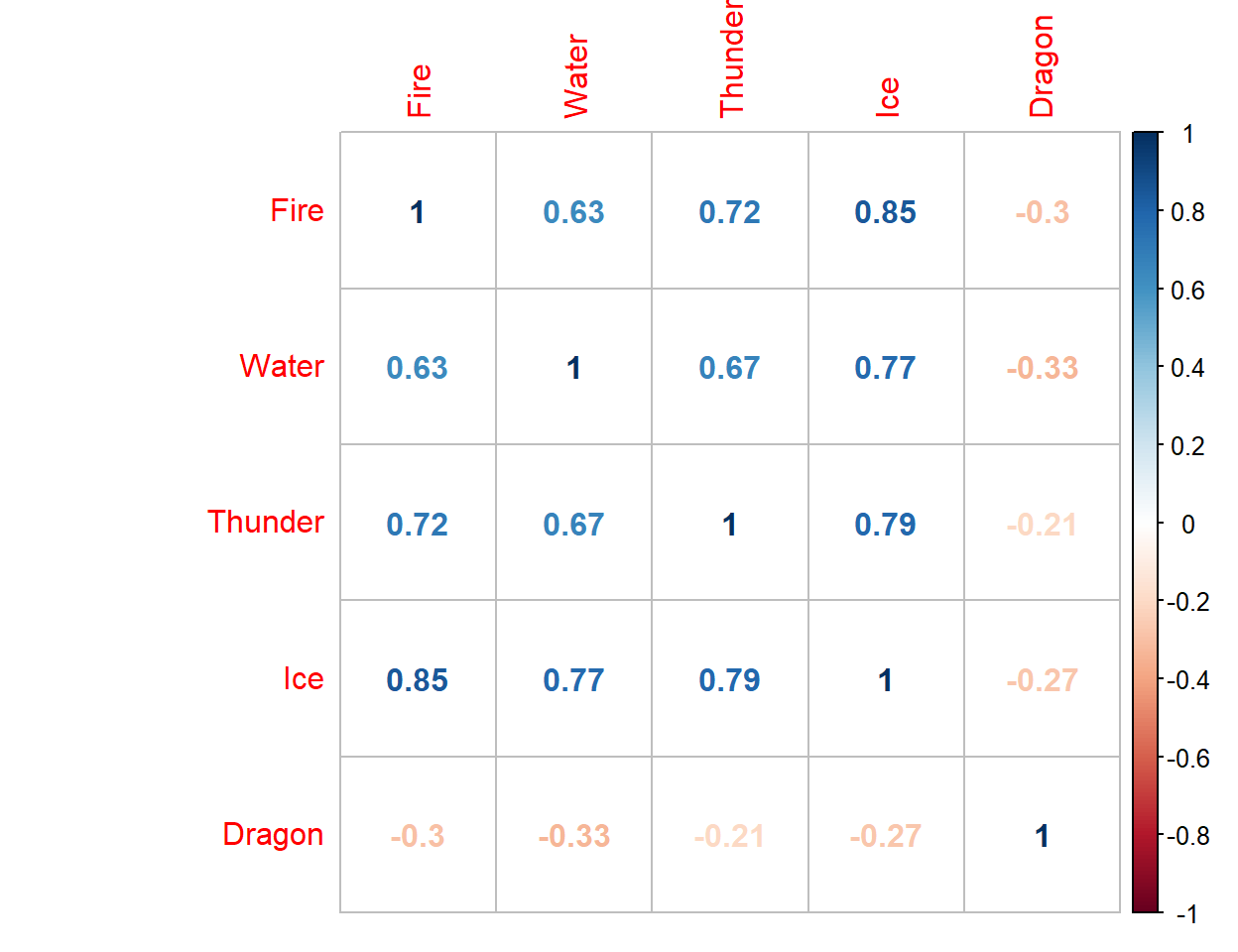
Non-Dragon Element Analysis
Here, I test whether or not removing the dragon element from the data will lead to any different clustering solutions. Furthermore, I've removed the four monsters that were found in cluster 2, because they seem to have oddly high elemental weakness values relative to rest of the monsters. In other words, these monsters could be considered the 'super weak' monsters and don't have much elemental idiosyncrasy. The results below show that even with these removals, the best solution seems to be 2 clusters. However, it could be argued that 3 clusters could also be used, because 9 indices of fit proposed the 2 cluster solution whereas 8 proposed a 3 cluster solution. Let's compare the 2 cluster and 3 cluster solutions!
MonsterChart_ND <- MonsterChart %>%
  select(-c(Dragon, Family)) %>%
  mutate(Cluster = NB_clust$Best.partition) %>%
  filter(Cluster != 2)

#MODEL COMPARISONS
  # function to compute total within-cluster sum of square (elbow method)
  fviz_nbclust(MonsterChart_ND[,2:5], kmeans, method = "wss")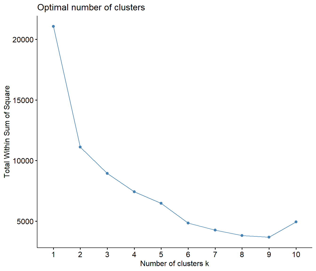
  # silhouette method
  fviz_nbclust(MonsterChart_ND[,2:5], kmeans, method = "silhouette")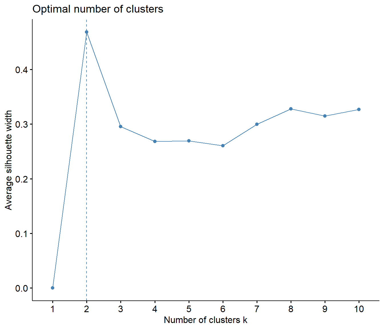
  diss_matrix <- dist(MonsterChart_ND[,2:5], method = "euclidean", diag = FALSE)
  NB_clust <- NbClust(MonsterChart_ND[,2:5], diss = diss_matrix, distance = NULL, min.nc = 2,
             max.nc = 10, method = "complete", index = "alllong")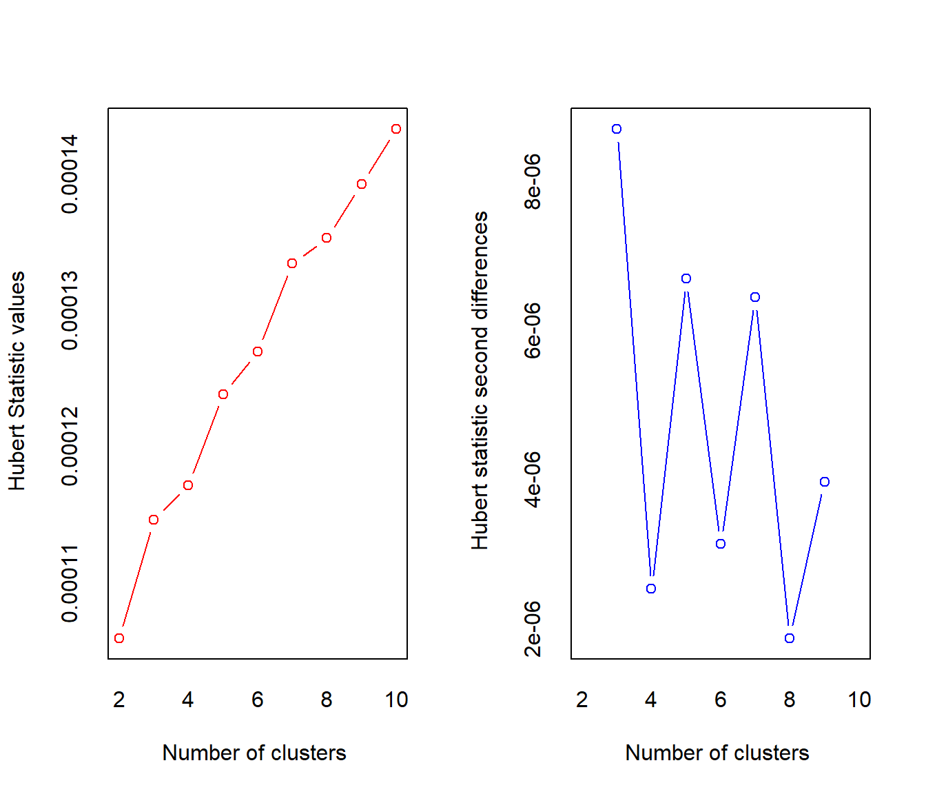
## *** : The Hubert index is a graphical method of determining the number of clusters.
##                 In the plot of Hubert index, we seek a significant knee that corresponds to a
##                 significant increase of the value of the measure i.e the significant peak in Hubert
##                 index second differences plot.
## 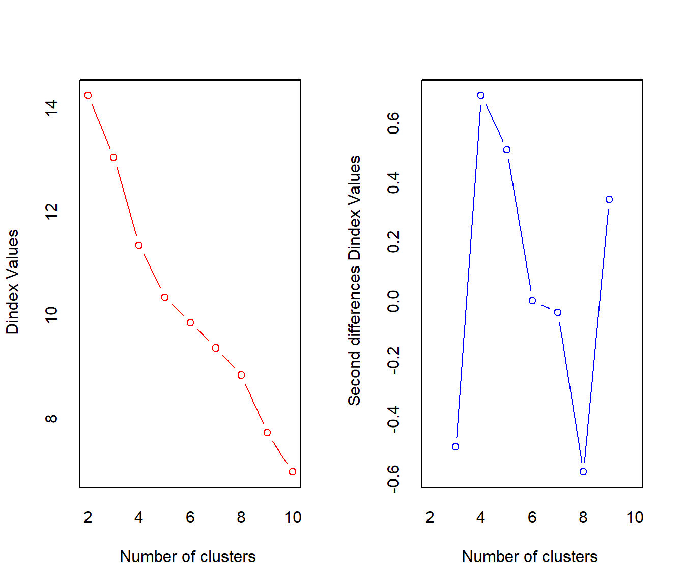
## *** : The D index is a graphical method of determining the number of clusters.
##                 In the plot of D index, we seek a significant knee (the significant peak in Dindex
##                 second differences plot) that corresponds to a significant increase of the value of
##                 the measure.
##
## *******************************************************************
## * Among all indices:
## * 9 proposed 2 as the best number of clusters
## * 8 proposed 3 as the best number of clusters
## * 3 proposed 4 as the best number of clusters
## * 1 proposed 5 as the best number of clusters
## * 1 proposed 6 as the best number of clusters
## * 1 proposed 8 as the best number of clusters
## * 4 proposed 10 as the best number of clusters
##
##                    ***** Conclusion *****
##
## * According to the majority rule, the best number of clusters is  2
##
##
## *******************************************************************
Two-Cluster Solution (Dragon element & Super weak removed) Results
A clearer pattern is beginning to show in the two cluster solution. Most of the small monsters are now loading into the second cluster, while the remaining large monsters are loading into the first cluster. Perhaps this warrants one additional anlaysis with the small monsters removed.
 MH_cluster2 <- kmeans(MonsterChart_ND[,2:5],2, nstart = 25)


#Incorporate cluster partition into data set
  MonsterChart_ND %>%
    mutate(Cluster_new = MH_cluster2$cluster) %>%
    mutate(Cluster_Name = ifelse(Cluster_new == 1, "Cluster 1", "Cluster 2")) %>%
    ggplot(aes(x = reorder(Monster, Cluster_new), y = Cluster_Name)) +
    geom_tile(aes(fill = Cluster_Name), colour = "white") +
    coord_equal(ratio = 0.9) +
    scale_fill_manual(values = c("black", "violet")) +
    theme(axis.text.y = element_blank(),
          axis.text.x = element_text(face = "bold", size = 10, angle = 90, hjust = 1),
            axis.line = element_blank(), axis.title.y = element_blank(), axis.title.x = element_blank(),
            axis.ticks.y = element_blank(), axis.ticks.x = element_blank(),
            axis.ticks.length = unit(0.2, "cm"),
            panel.grid.major = element_blank(), panel.grid.minor = element_blank(),
            panel.border = element_blank(), panel.background = element_blank(),
            legend.title = element_blank(), legend.direction = "horizontal",
            legend.key.size = unit(0.5,"cm"), legend.spacing.x = unit(0.4, "cm"),
legend.position = c(0.5, 1.5)) 
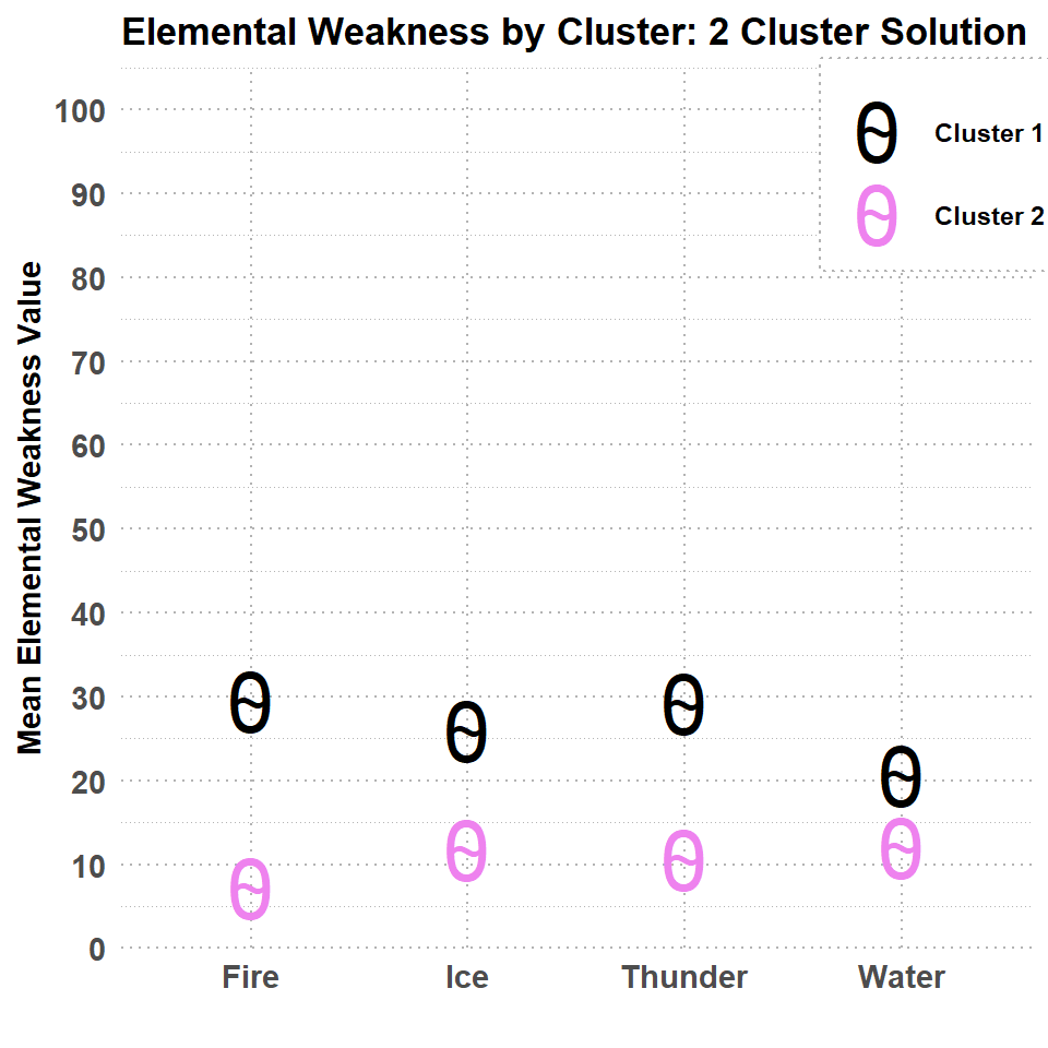
As can be seen in the table below, the elemental weakness pattern between the two clusters is a little bit more nuanced.
Cluster2_means <- as.data.frame(MH_cluster2$centers)

Cluster2_means <- Cluster2_means %>%
  mutate(Cluster = c("Cluster 1", "Cluster 2")) %>%
  select(Cluster, Fire, Water, Thunder, Ice)

pander(Cluster2_means, style = 'rmarkdown')| Cluster | Fire | Water | Thunder | Ice |
|---|---|---|---|---|
| Cluster 1 | 29.42 | 20.67 | 29.17 | 26 |
| Cluster 2 | 7.257 | 12.06 | 10.6 | 11.71 |
The differences between the cluster means become more apparent in the plot below.
#Dinasaur egg plot
size1 <- 10
size2 <- size1*0.7
Cluster2_means %>%
  gather(2:5, key = "Element", value = "Cluster Mean") %>%
  ggplot(aes(x = Element, y = `Cluster Mean`, color = Cluster, shape = Cluster)) +
  geom_point(size=size1, shape = 48) +
  geom_point(size=size2, shape = 126) +
  scale_color_manual(values = c("black", "violet")) +
  scale_y_continuous(breaks = seq(0,100,10), limits = c(0,105), expand = c(0,0)) +
  ylab("Mean Elemental Weakness Value") +
  xlab("") +
  ggtitle("Elemental Weakness by Cluster: 2 Cluster Solution") +
  theme_minimal() +
  theme(
    panel.grid = element_line(color = "grey70", linetype = "dotted"),
    legend.position = c(0.9,0.89),
    legend.background = element_rect(fill = "white", color = "grey70", linetype = "dotted"),
    legend.text = element_text(face = "bold"),
    legend.title = element_blank(),
    axis.text = element_text(face = "bold", size = 11),
      axis.title = element_text(face = "bold"),
   title = element_text(face = "bold")
  )
Two-Cluster (Dragon element & Super weak removed) Conclusion
The results from this two cluster solution are interesting. The first cluster seems to include monsters that have overall more weakness to the elements, particularly for Fire, Thunder and Ice. Cluster two has overall less elemental weakness than cluster 1, and the primary weaknesses seem to be for Water, Thunder, and Ice (though Fire is not that much different). Let's see how this compares to the 3 cluster solution.
Three-Cluster Solution (Dragon element & Super weak removed) Results
The story gets thicker! This is more difficult to interpret what is going on just based on the monsters in each cluster. Generally, clusters 1 and 3 seem to have more large monsters, while cluster 2 is comprised mostly of small monsters. Notably, the rathalos and rathian family are all grouped into cluster 3, which is what should be expected given their similarities.
MH_cluster3 <- kmeans(MonsterChart_ND[,2:5],3, nstart = 25)

#Incorporate cluster partition into data set
  MonsterChart_ND %>%
    mutate(Cluster = MH_cluster3$cluster) %>%
    mutate(Cluster_Name = case_when(Cluster == 1 ~ "Cluster 1",
                                    Cluster == 2 ~ "Cluster 2",
                                    Cluster == 3 ~ "Cluster 3")) %>%
    ggplot(aes(x = reorder(Monster, Cluster), y = Cluster_Name)) +
    geom_tile(aes(fill = Cluster_Name), colour = "white") +
    coord_equal(ratio = 0.9) +
    scale_fill_manual(values = c("black", "violet", "skyblue")) +
    theme(axis.text.y = element_blank(),
          axis.text.x = element_text(face = "bold", size = 10, angle = 90, hjust = 1),
            axis.line = element_blank(), axis.title.y = element_blank(), axis.title.x = element_blank(),
            axis.ticks.y = element_blank(), axis.ticks.x = element_blank(),
            axis.ticks.length = unit(0.2, "cm"),
            panel.grid.major = element_blank(), panel.grid.minor = element_blank(),
            panel.border = element_blank(), panel.background = element_blank(),
            legend.title = element_blank(), legend.direction = "horizontal",
            legend.key.size = unit(0.5,"cm"), legend.spacing.x = unit(0.2, "cm"),
            legend.position = c(0.5, 1.5))
If we take a look at the cluster means, we can see that there is even more uniqueness to the pattern of elemental weakness between the three clusters. Cluster 2 seems to have on average more elemental weakness overall. Clusters 1 and 3 are similar, but seem to be differentiated by their weaknesses to Ice, Thunder, and Water.
Cluster3_means <- as.data.frame(MH_cluster3$centers)

Cluster3_means <- Cluster3_means %>%
  mutate(Cluster = c("Cluster 1", "Cluster 2", "Cluster 3")) %>%
  select(Cluster, Fire, Water, Thunder, Ice)

pander(Cluster3_means, style = 'rmarkdown')| Cluster | Fire | Water | Thunder | Ice |
|---|---|---|---|---|
| Cluster 1 | 7.526 | 5.368 | 13 | 9.105 |
| Cluster 2 | 33.5 | 20.3 | 29.2 | 26.7 |
| Cluster 3 | 7.167 | 20.28 | 10.11 | 15.67 |
As with the previous analyses, the pattern of elemental weakness can be more easily seen in the plot below. Note: The icons in this graph have been jittered to reduce overlap.
#Dinasaur egg plot
size1 <- 10
size2 <- size1*0.7
Cluster3_means %>%
gather(2:5, key = "Element", value = "Cluster Mean") %>%
ggplot(aes(x = Element, y = `Cluster Mean`, color = Cluster, shape = Cluster)) +
geom_point(size=size1, shape = 48, position = position_dodge(width = 0.4)) +
geom_point(size=size2, shape = 126, position = position_dodge(width = 0.4)) +
scale_color_manual(values = c("black", "violet", "skyblue")) +
scale_y_continuous(breaks = seq(0,100,10), limits = c(0,105), expand = c(0,0)) +
ylab("Mean Elemental Weakness Value") +
xlab("") +
ggtitle("Elemental Weakness by Cluster: 3 Cluster Solution") +
theme_minimal() +
theme(
panel.grid = element_line(color = "grey70", linetype = "dotted"),
legend.position = c(0.9,0.84),
legend.background = element_rect(fill = "white", color = "grey70", linetype = "dotted"),
legend.text = element_text(face = "bold"),
legend.title = element_blank(),
axis.text = element_text(face = "bold", size = 11),
axis.title = element_text(face = "bold"),
title = element_text(face = "bold")
)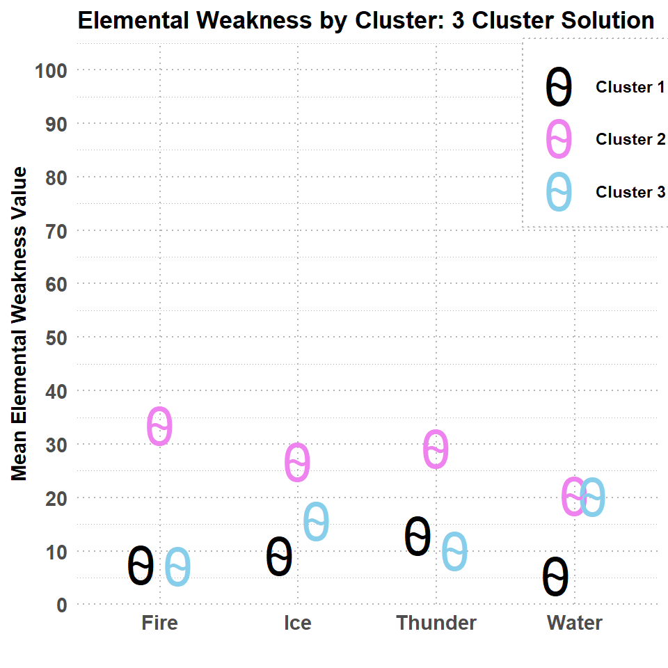 ###Three-Cluster Solution (Dragon element & Super weak removed) Conclusion The three cluster solution produced some neat results. Cluster 1 seems to reflect a group of large monsters that are relatively weak to Water and Ice. Cluster 2 seems to be a grouping of small monsters who are generally much weaker to all elemental damage. The monsters in cluster 3 are all large monsters except for Barnos, and have the highest average elemental resistances. However, cluster three does show slightly more weakness to thunder relative to cluster 1, though the difference is small.
No Small Monsters
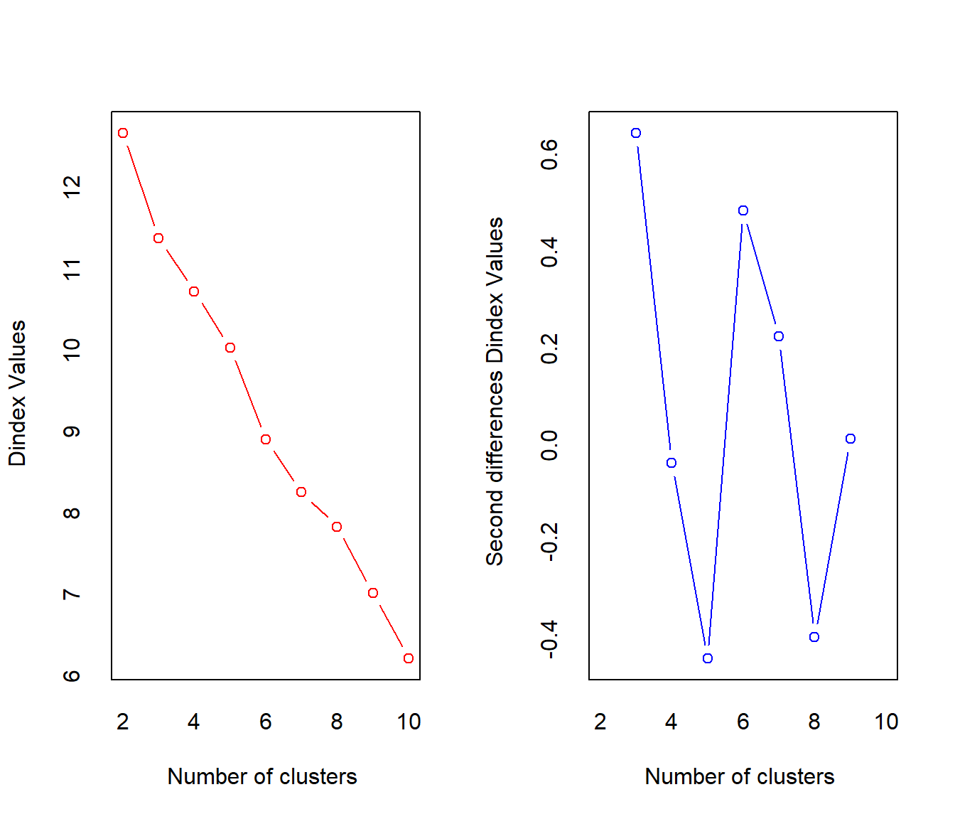
The last analysis is for only large monsters. The dragon element has also been reintroduced into the analysis. Suprisingly, the model fit comparisons proposed that a 10 cluster solution would be most ideal. A two cluster and three cluster solution seem to also be probable based on the model comparisons.
MonsterChart_LM <- MonsterChart %>%
  filter(Family != "Small Monster")

#MODEL COMPARISONS
  # function to compute total within-cluster sum of square (elbow method)
  fviz_nbclust(MonsterChart_LM[,3:7], kmeans, method = "wss")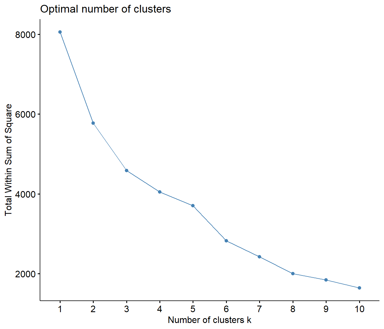
  # silhouette method
  fviz_nbclust(MonsterChart_LM[,3:7], kmeans, method = "silhouette")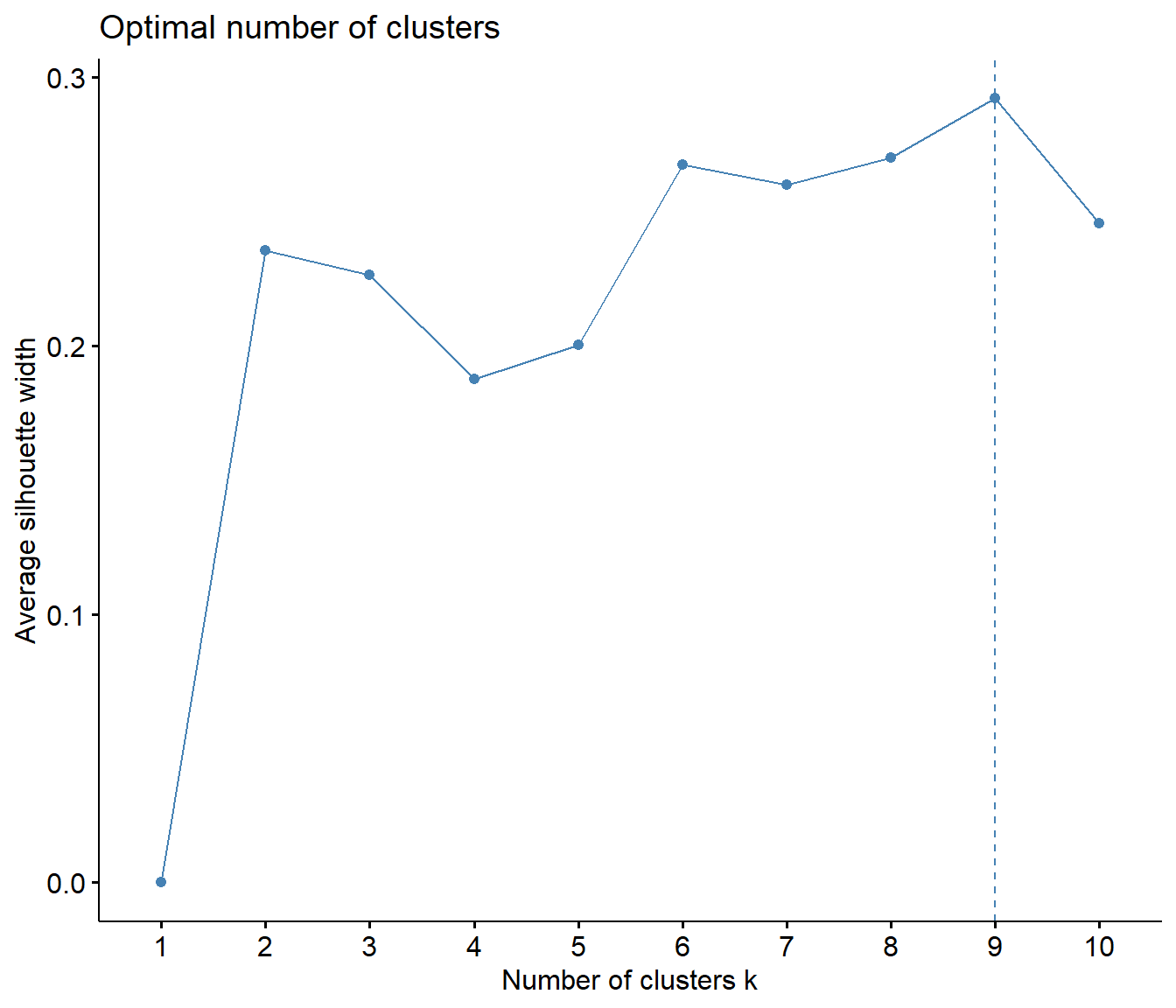
  diss_matrix <- dist(MonsterChart_LM[,3:7], method = "euclidean", diag = FALSE)
  NB_clust <- NbClust(MonsterChart_LM[,3:7], diss = diss_matrix, distance = NULL, min.nc = 2,
             max.nc = 10, method = "complete", index = "alllong")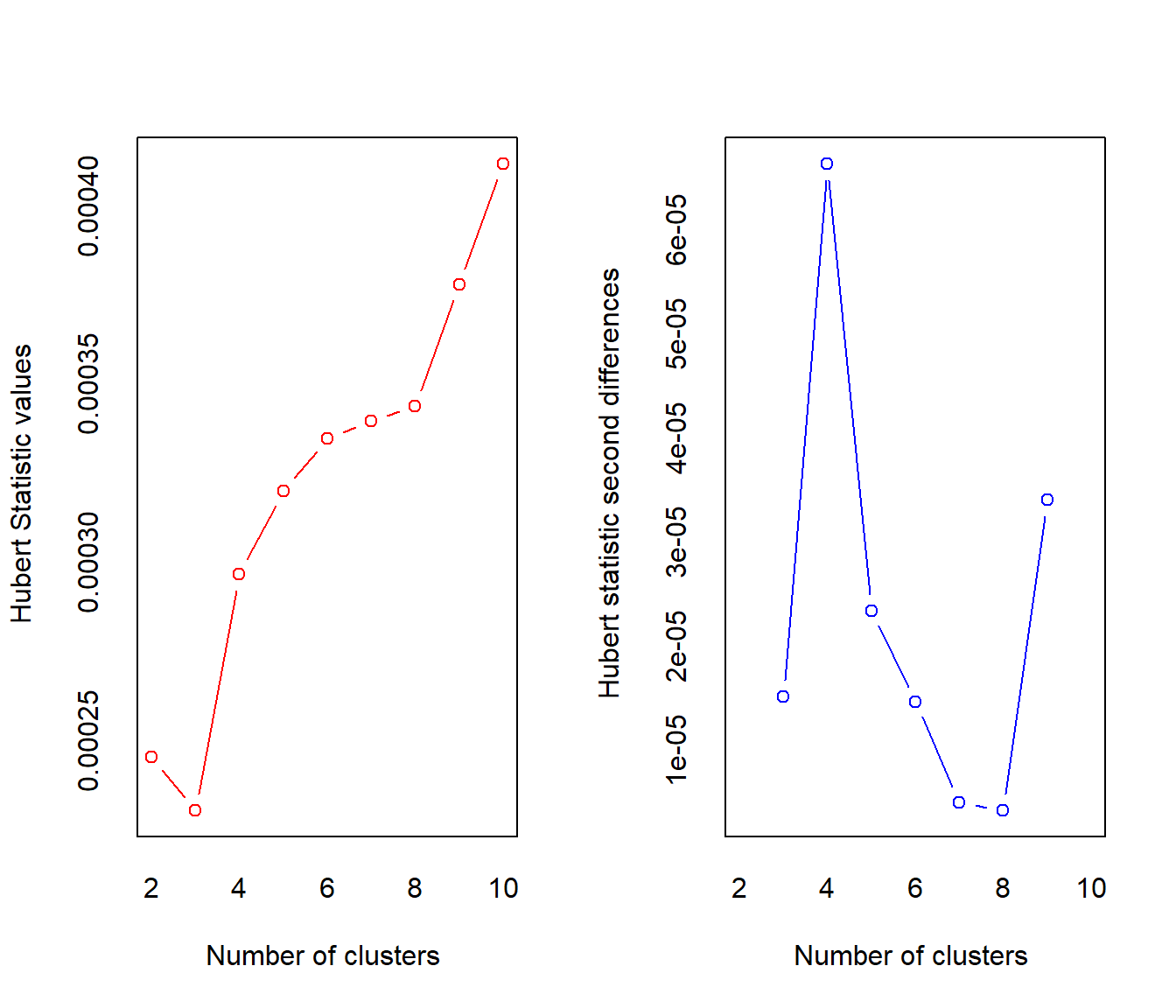
## *** : The Hubert index is a graphical method of determining the number of clusters.
##                 In the plot of Hubert index, we seek a significant knee that corresponds to a
##                 significant increase of the value of the measure i.e the significant peak in Hubert
##                 index second differences plot.
## 
## *** : The D index is a graphical method of determining the number of clusters.
##                 In the plot of D index, we seek a significant knee (the significant peak in Dindex
##                 second differences plot) that corresponds to a significant increase of the value of
##                 the measure.
##
## *******************************************************************
## * Among all indices:
## * 7 proposed 2 as the best number of clusters
## * 7 proposed 3 as the best number of clusters
## * 4 proposed 9 as the best number of clusters
## * 9 proposed 10 as the best number of clusters
##
##                    ***** Conclusion *****
##
## * According to the majority rule, the best number of clusters is  10
##
##
## *******************************************************************
10 Cluster Solution (No Small Monsters) Results
The 10 Cluster Solution provides some neat results! Firstly, a quick moment of silence for the poor Barroth, who is all alone in cluster 4.
  MonsterChart_LM %>%
    mutate(Cluster = NB_clust$Best.partition) %>%
    ggplot(aes(x = reorder(Monster, Cluster), y = Cluster)) +
    geom_tile(aes(fill = factor(Cluster)), colour = "white") +
    coord_equal(ratio = 0.9) +
    labs(fill = "Cluster") +
    #scale_fill_manual(values = c("black", "violet", "skyblue")) +
    theme(axis.text.y = element_blank(),
          axis.text.x = element_text(face = "bold", size = 10, angle = 90, hjust = 1),
            axis.line = element_blank(), axis.title.y = element_blank(), axis.title.x = element_blank(),
            axis.ticks.y = element_blank(), axis.ticks.x = element_blank(),
            axis.ticks.length = unit(0.2, "cm"),
            panel.grid.major = element_blank(), panel.grid.minor = element_blank(),
            panel.border = element_blank(), panel.background = element_blank(),
            legend.direction = "horizontal",legend.key.size = unit(0.5,"cm"),
legend.spacing.x = unit(0.4, "cm"), legend.position = c(0.5, 0.9)) 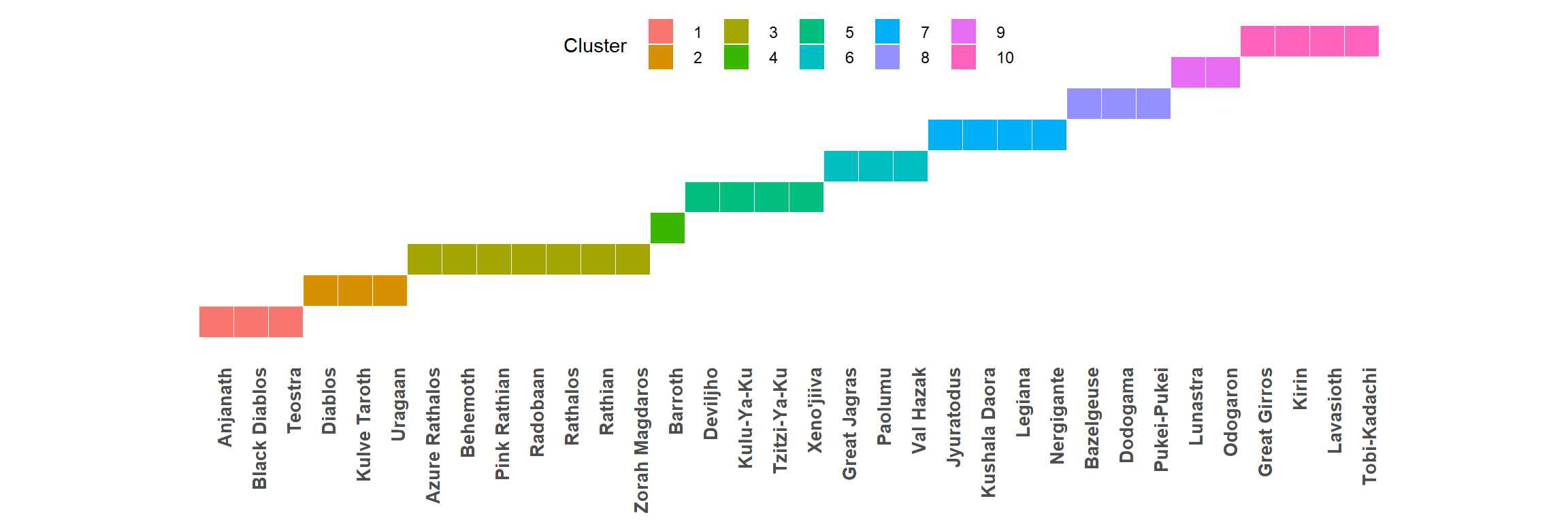
Here are the elemental weakness means for each cluster. There are quite neat patterns to be seen in some of these clusters! For instance, cluster 2 comprises of monsters who are extremely weak to Water,while cluster 3 is a unique combination of monsters that are equally weak to Water, Ice, and Dragon elements.
#Cluster means
MH_cluster10_LM <- kmeans(MonsterChart_LM[,3:7],10, nstart = 25)
Cluster10_means <- as.data.frame(MH_cluster10_LM$centers)
Cluster10_means <- Cluster10_means %>%
  mutate(Cluster = 1:10) %>%
  select(Cluster, Fire, Water, Thunder, Ice, Dragon)

pander(Cluster10_means, style = 'rmarkdown')| Cluster | Fire | Water | Thunder | Ice | Dragon |
|---|---|---|---|---|---|
| 1 | 11.67 | 14.33 | 15 | 13.5 | 15.67 |
| 2 | 12 | 40 | 0 | 14 | 9 |
| 3 | 2 | 20.33 | 9 | 19.67 | 20 |
| 4 | 8.25 | 6.5 | 15 | 2.5 | 7.5 |
| 5 | 10.5 | 19 | 1.5 | 9.75 | 4.5 |
| 6 | 0 | 20.67 | 7.667 | 17.67 | 3 |
| 7 | 0 | 7.8 | 9.4 | 8 | 19.8 |
| 8 | 2.667 | 6.333 | 20.33 | 12.33 | 8.333 |
| 9 | 2 | 4.5 | 7 | 19.5 | 7 |
| 10 | 19.67 | 1.333 | 11 | 9.333 | 7.667 |
10 Cluster Solution (No Small Monsters) Conclusion
The 10 cluster solution showed a remarkable amount of idiosyncrasy between the clusters. Based on the table, several patterns of elemental weakneses were represented. Some clusters were quite straightforward, like cluster 2 whose monsters were severely weak to Water, while others were a bit more difficult to interpret with respect to the other clusters. Regardless, this last analysis shows quite a bit of cool and interesting things. Perhaps the most notable takeaway is that the monster hunter team has really put together a great group of large monsters, who fit into several different types of elemental weakness patterns.
Overall Conclusion
The results from the analyses above all provide a unique story. The monsters of Monster Hunter World have now been categorized based on their elemental weaknesses, which to my knowledge has not previously been done. There are of course, alternative clustering algorithms that could have been used which could have produced different results. Overall, there seems to be a few takeaways from all of this. First, the small monsters of MHW are quite different than the large monsters. Their elemental weaknesses were overall just far more than the large monsters. Second, MHW monsters can be classified into relatively few clusters if using all or most of the monsters in the game. Lastly, within the large monster group, there is a wild amount of uniqueness with respect to elemental weaknesses.